NFSD: Noise Free Score Distillation

Oren Katzir^*¹, Or Patashnik^*¹, Daniel Cohen-Or¹, Dani Lischinski²

¹Tel-Aviv University, ²The Hebrew University of Jerusalem

^*Denotes Equal Contribution

Abstract

Score Distillation Sampling (SDS) has emerged as the de facto approach for text-to-content generation in non-image domains. In this paper, we reexamine the SDS process and introduce a straightforward interpretation that demystifies the necessity for large Classifier-Free Guidance (CFG) scales, rooted in the distillation of an undesired noise term. Building upon our interpretation, we propose a novel Noise-Free Score Distillation (NFSD) process, which requires minimal modifications to the original SDS framework. Through this streamlined design, we achieve more effective distillation of pre-trained text-to-image diffusion models while using a nominal CFG scale. This strategic choice allows us to prevent the over-smoothing of results, ensuring that the generated data is both realistic and complies with the desired prompt. To demonstrate the efficacy of NFSD, we provide qualitative examples that compare NFSD and SDS, as well as several other methods.

Some results obtained by NFSD

Our Approach

Given a set of parameters $\theta$ of a differentiable parametric image generator $g$, a condition $y$ and a pretrained diffusion model $\unet$, we wish to optimize $\theta$ by distillation from the CFG score: $$ \epredcfg = \unet(\z_t ; y=\varnothing, t) + s \left(\epred - \unet(\z_t ; y=\varnothing, t) \right). $$ To gain a better understanding of SDS, it is helpful to examine the decomposition of $\epredcfg$ into several intuitively interpretable components.

Score Decomposition

condition direction. The difference $\dirc = \epred - \epuncond$ may be thought of as the direction that steers the generated image towards alignment with the condition $y$. The condition direction $\delta_c$ (demonstrated below) is empirically observed to be aligned with the condition and uncorrelated with the added noise $\epsilon$.

noise and in-domain directions. Rewriting the CFG score using the condition direction $\dirc$ defined above, we obtain: $$ \epredcfg = \epuncond + s(\epred - \epuncond) = \epuncond + s\dirc. $$

The unconditional term $\epuncond$ is expected to predict the noise $\epsilon$ that was added to an image $\x \sim p_{\text{data}}$ to produce $\z_t$. However, in SDS, $\z_t$ is obtained by adding noise to an out-of-distribution (OOD) rendered image $\x = g(\theta)$, which is not sampled from $p_{\text{data}}$. Thus, we can think of $\epuncond$ as a combination of two components, $\epuncond = \dirr + \dirn$.

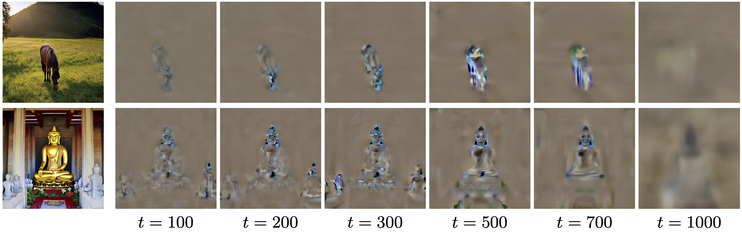
We attempt to visualize the two components by examining the difference between two unconditional predictions $\epsilon_\phi(\z_{t}(\x_{\textrm{ID}}); \varnothing,t)$ and $\epsilon_\phi(\z_{t}(\x_{\textrm{OOD}}); \varnothing,t)$, where $\z_{t}(\x_{\textrm{ID}})$ and $\z_{t}(\x_{\textrm{OOD}})$ are noised in-domain and out-of-domain images, respectively, that depict the same content and are added the same noise $\epsilon$. Intuitively, while $\epsilon_\phi(\z_{t}(\x_{\textrm{OOD}}); \varnothing,t)$ both removes noise ($\dirn$) and steers the sample towards the model's domain ($\dirr$), the prediction $\epsilon_\phi(\z_{t}(\x_{\textrm{ID}}))$ mostly just removes noise ($\dirn$), since the image is already in-domain. Thus, the difference between these predictions enables the sepeartion of $\dirn$ and $\dirr$.

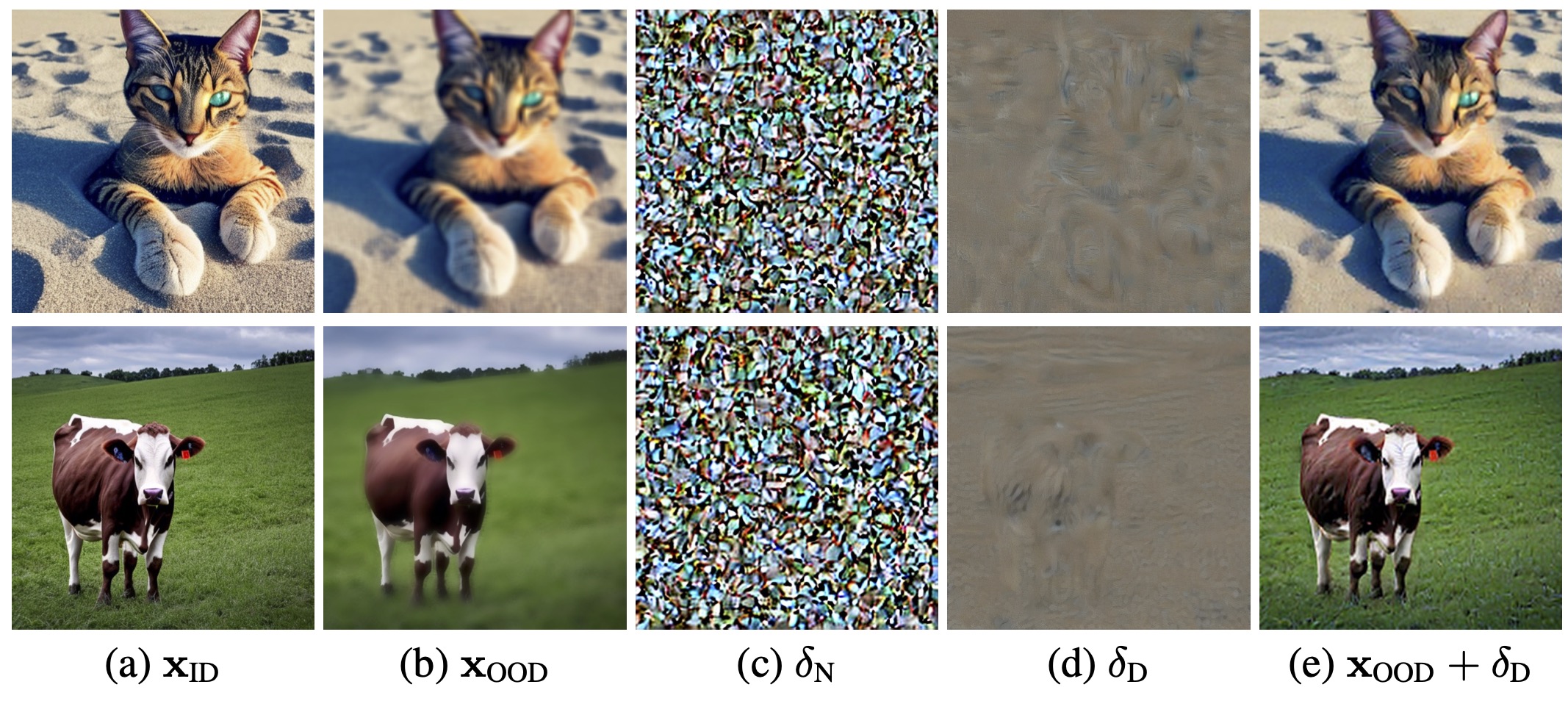
As can be seen, $\dirn$ indeed appears to consist of noise uncorrelated with the image content, while $\dirr$ is large in areas where the distortion is most pronounced and adding $\dirr$ to $\x_{\textrm{OOD}}$ effectively enhances the realism of the image (column (e)).

Noise Free Score Distillation

As discussed above, ideally only the $s\dirc$ and the $\dirr$ terms should be used to guide the optimization of the parameters $\theta$.

To extract $\dirr$, we distinguish between different stages in the backward (denoising) diffusion process.

For sufficiently small timestep values $t < 200$, $\dirn$ is rather small, and the score $\epuncond = \dirn + \dirr$ is increasingly dominated by $\dirr$.

As for the larger timestep values, $t \geq 200$, we propose to approximate $\dirr$ by the difference $\epuncond - \epneg$, where $\pneg =$ ``unrealistic, blurry, low quality, out of focus, ugly, low contrast, dull, dark, low-resolution, gloomy''. Here, we are making the assumption that $\delta_{C=\pneg} \approx -\dirr$, and thus $$ \epuncond - \epneg = \dirr + \dirn - (\dirr + \dirn + \delta_{C = \pneg}) \approx \dirr. $$

To conclude, we approximate $\dirr$ by $$ \dirr = \begin{cases} \epuncond , & \text{if } t < 200 \\ \epuncond - \unet(\z_t; y=\pneg,t), & \text{otherwise,} \end{cases} $$ and use the resulting $\dirc$ and $\dirr$ to define an alternative, $\textit{noise-free score distillation}$ loss $\Loss_\text{NFSD}$, whose gradients are used to optimize the parameters $\theta$, instead of $\grad{\theta}\Loss_\text{SDS}$: $$ \grad{\theta} \Loss_\text{NFSD} = w(t) \left(\dirr + s\dirc \right) \frac{\partial \x}{\partial \theta}. $$

Score Decomposition with respect to previous works

Our score decomposition formulation can be used to explain both SDS and previous works that were proposed to improve the SDS loss, which demonstrates the wide scope and applicability of our formulation.

Revisiting SDS with our interpertaion, $$ \grad{\theta} \Loss_\text{SDS} = w(t)(\epredcfg - \epsilon) \frac{\partial \x}{\partial \theta} = w(t)(\dirr + \dirn + s\dirc - \epsilon) \frac{\partial \x}{\partial \theta}. $$ Note that while both $\dirr$ and $\dirc$ are needed to steer the rendered image towards an in-domain image aligned with the condition $y$, the residual $\dirn - \epsilon$ is generally non-zero and noisy. Importantly, our decomposition explains the need for using a large CFG coefficient in SDS (e.g., $s=100$), as this enables the image-correlated $s\dirc$ term to dominate the loss, making the noisy residual $\dirn - \epsilon$ relatively negligible.

DDS propose an adaptation of the SDS loss for image editing task and is defined by $$ \grad{\theta} \Loss_\text{DDS} = \grad{\theta} \Loss_\text{SDS}(\z_t(\x), y) - \grad{\theta} \Loss_\text{SDS}(\tilde{\z}_t(\tilde{\x}), \tilde{y}), $$ where $\tilde{\z}_t(\tilde{\x}), \tilde{y}$ denote the noisy original input image and its corresponding prompt, respectively. Here $y$ denotes the prompt that describes the edit, and $\x, \tilde{\x}$ are noised with the same noise $\epsilon$. Incorporating our score decomposition yields $$ \grad{\theta} \Loss_\text{DDS} = w(t)(\dirr + \dirn + s\delta_{C_\text{edit}} - \epsilon) - w(t)(\dirr + \dirn + s\delta_{C_\text{orig}} - \epsilon) = w(t) s(\delta_{C_\text{edit}} - \delta_{C_\text{orig}}). $$ Our formulation helps to understand the high-quality results achieved by DDS: the residual component which makes the results in SDS over-smoothed and over-saturated is cancelled out. Moreover, since the optimization is initialized with an in-domain image, the $\dirr$ component is not effectively needed and cancelled out. The remaining direction is the one relevant to the difference between the original prompt and the new one.

ProlificDreamer tackle the generation task, and propose the VSD loss, which successfully alleviates the over-smoothed and over-saturated results obtained by SDS. In VSD, alongside the pretrained diffusion model $\unet$, another diffusion model $\epsilon_\text{LoRA}$ is trained during the optimization process. The $\epsilon_\text{LoRA}$ model is initialized with the weights of $\unet$, and during the optimization process it is fine-tuned with rendered images $\x = g(\theta)$. Effectively, the rendered images during the optimization are out-of-domain for the original pretrained model distribution, but are in-domain for $\epsilon_\text{LoRA}$. Hence, the gradients of the VSD loss are defined as $$ \grad{\theta} \Loss_\text{VSD} = w(t) \left(\epredcfgx - \epsilon_\text{LoRA}(\z_t(\x);y,t,c \right) \frac{\partial \x}{\partial \theta}, $$ where $c$ is another condition that is added to $\epsilon_\text{LoRA}$ and represents the camera viewpoint of the rendered image $\x$. Viewed in terms of our score decomposition, since $\epsilon_\text{LoRA}$ is fine-tuned on $\x$, both $\dirc$ and $\dirr$ are approximately $0$, thus it simply predicts $\dirn$. Therefore, $\grad{\theta} \Loss_\text{VSD}$ can be written as $$ \grad{\theta} \Loss_\text{VSD} = w(t) (\dirr + \dirn + s\dirc - \dirn) \frac{\partial \x}{\partial \theta} = w(t) (\dirr + s\dirc) \frac{\partial \x}{\partial \theta}, $$ i.e., it approximates exactly the same terms as our NFSD. It should be noted that unlike our approach, VSD has a considerable computational overhead of fine-tuning the additional diffusion model during the optimization process.

Comparison

2D image generation

NFSD optimization of the latent code of Stable Diffusion is able to produce more pleasing results in which the object is clear, the background is detailed, and the image looks more realistic, even when using a CFG value of 7.5. SDS optimization with a nominal CFG scale (7.5) yields oversmoothed images (top row), while using a high CFG scale (100) generates the main object but lacks background details and occasionally introduces aritfacts (middle row).

Text-to-NeRF synthesis

For generation of 3D objects, NFSD allows better distillation and typically generates fewer fine details.

Comparison with related methods

For each of the methods we compare to results that were reported by the authors. As can be seen, our method achieves comparable or better results, while being significantly simpler than most of these methods.

BibTeX

@misc{katzir2023noisefree,
      title={Noise-Free Score Distillation}, 
      author={Oren Katzir and Or Patashnik and Daniel Cohen-Or and Dani Lischinski},
      year={2023},
      eprint={2310.17590},
      archivePrefix={arXiv},
      primaryClass={cs.CV}
}